Benchmarks
Last synced benchmark assets: 2026-05-14T15:39:50.351535+00:00
CPU: x86_64 with 2 logical cores
Platform: Linux-6.8.0-1044-azure-x86_64-with-glibc2.39
Python: 3.12.1, NumPy: 2.3.5, SciPy: 1.16.3, Optyx: 1.3.1
1 Benchmarks
Optyx includes a comprehensive benchmark suite measuring end-to-end performance including variable creation, problem setup, constraint construction, and solving. All benchmarks compare against raw SciPy (which has no build phase).
This page renders directly from synced artifacts in docs/assets/benchmarks/:
benchmark_results.jsonfor structured tables and summary valuesbenchmark_metadata.jsonfor machine and dependency metadatabenchmark_output.txtfor the raw console transcript.pngplots copied from the latest benchmark run
1.1 Quick Start
# Run all benchmark tests
uv run pytest benchmarks/ -v

# Generate performance analysis plots and sync docs assets automatically
uv run python benchmarks/run_benchmarks.pyAll benchmarks measure total time including:
- Variable creation
- Problem setup
- Constraint construction
- Cold solve (first solve, includes compilation)
- Warm solve (cached subsequent solves)
1.2 Performance Summary
| Problem Type | Size | Cold Overhead | Warm Overhead | Notes |
|---|---|---|---|---|
| LP | n=50 | 2.9x | 1.3x | Near-parity with SciPy linprog |
| LP | n=500 | 0.4x | 0.4x | Near-parity with SciPy linprog |
| LP | n=5000 | 2.3x | 1.1x | Scales to large LPs while staying near parity |
| NLP | n=50 | 1.8x | 1.3x | Autodiff overhead on a trivially simple objective |
| NLP | n=500 | 1.2x | 0.7x | Autodiff overhead on a trivially simple objective |
| NLP | n=5000 | 1.6x | 1.1x | Simple quadratic; SciPy converges almost instantly |
| CQP | n=50 | 1.8x | 1.1x | O(1) Jacobian compilation for vectorized constraints |
| CQP | n=500 | 0.7x | 0.5x | O(1) Jacobian compilation for vectorized constraints |
| CQP | n=5000 | 1.2x | 1.0x | Exact Jacobians keep constrained solves near parity |
| MILP | n=50 | 2.1x | 1.6x | Near-parity with SciPy milp |
| MILP | n=500 | 2.0x | 1.8x | Near-parity with SciPy milp |
| MILP | n=5000 | 1.6x | 1.1x | Scales to large binary knapsack problems |
Key Insight: Cold solves include one-time compilation. Warm solves (repeated optimization with cached structure) achieve near-parity with raw SciPy for LP, CQP, and MILP. NLP overhead reflects autodiff costs on trivially simple benchmarks — for complex nonlinear problems, automatic differentiation provides significant modeling advantages.
1.3 LP Scaling: VectorVariable vs Loop-Based
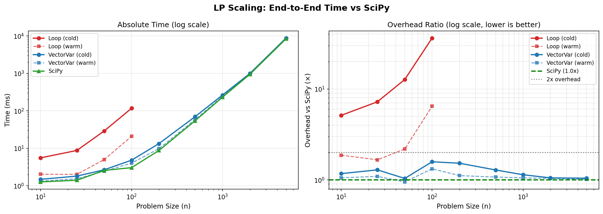
1.3.1 Loop-Based Variables (n ≤ 500)
| n | Build | Cold Solve | Warm Solve | SciPy | Cold Overhead | Warm Overhead |
|---|---|---|---|---|---|---|
| 10 | 0.5ms | 188.4ms | 2.1ms | 1.3ms | 140.6x | 1.6x |
| 25 | 1.2ms | 12.4ms | 1.9ms | 1.5ms | 8.9x | 1.2x |
| 50 | 3.3ms | 48.0ms | 2.3ms | 1.9ms | 27.5x | 1.2x |
| 100 | 13.1ms | 126.7ms | 4.8ms | 4.2ms | 33.2x | 1.1x |
| 200 | 58.1ms | 540.2ms | 8.8ms | 9.9ms | 60.2x | 0.9x |
| 500 | 590.1ms | 10,711.4ms | 120.6ms | 111.1ms | 101.8x | 1.1x |
Loop-based variable construction creates O(n²) expression tree nodes, causing exponential compilation time. Use VectorVariable for n > 50.
1.3.2 VectorVariable (n ≤ 5,000)
| n | Build | Cold Solve | Warm Solve | SciPy | Cold Overhead | Warm Overhead |
|---|---|---|---|---|---|---|
| 10 | 0.1ms | 3.0ms | 2.3ms | 2.1ms | 1.5x | 1.1x |
| 25 | 0.2ms | 2.5ms | 4.8ms | 3.2ms | 0.8x | 1.5x |
| 50 | 0.3ms | 8.1ms | 3.7ms | 2.9ms | 2.9x | 1.3x |
| 100 | 0.6ms | 24.8ms | 8.0ms | 5.8ms | 4.4x | 1.4x |
| 200 | 2.9ms | 23.6ms | 25.7ms | 19.1ms | 1.4x | 1.3x |
| 500 | 7.8ms | 121.1ms | 118.1ms | 320.7ms | 0.4x | 0.4x |
| 1000 | 8.1ms | 929.1ms | 311.5ms | 255.3ms | 3.7x | 1.2x |
| 2000 | 6.5ms | 1,600.5ms | 1,262.9ms | 1,109.1ms | 1.4x | 1.1x |
| 5000 | 12.9ms | 22,523.4ms | 10,496.0ms | 9,754.7ms | 2.3x | 1.1x |
VectorVariable achieves parity or better than raw SciPy for warm solves at all scales. Cold solve overhead is minimal due to one-time compilation.
1.4 NLP Scaling: Unconstrained Optimization
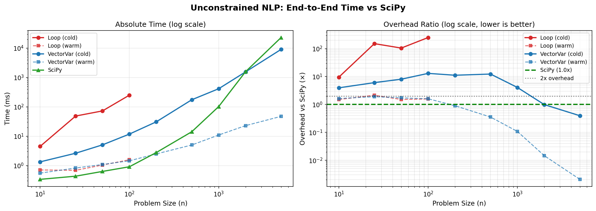
Objective: min Σx²ᵢ - Σxᵢ (optimal at x* = 0.5)
1.4.1 VectorVariable with x.dot(x) - x.sum()
| n | Build | Cold Solve | Warm Solve | SciPy | Cold Overhead | Warm Overhead |
|---|---|---|---|---|---|---|
| 10 | 0.0ms | 0.7ms | 0.3ms | 0.2ms | 3.3x | 1.3x |
| 25 | 0.0ms | 0.4ms | 0.3ms | 0.2ms | 2.0x | 1.3x |
| 50 | 0.0ms | 0.5ms | 0.4ms | 0.3ms | 1.8x | 1.3x |
| 100 | 0.0ms | 0.5ms | 0.3ms | 0.3ms | 1.9x | 1.0x |
| 200 | 0.0ms | 0.6ms | 0.4ms | 0.2ms | 3.2x | 2.1x |
| 500 | 0.0ms | 0.5ms | 0.3ms | 0.4ms | 1.2x | 0.7x |
| 1000 | 0.0ms | 0.6ms | 0.3ms | 0.3ms | 2.2x | 1.2x |
| 2000 | 0.0ms | 0.5ms | 0.5ms | 0.6ms | 1.0x | 0.8x |
| 5000 | 0.0ms | 0.8ms | 0.6ms | 0.5ms | 1.6x | 1.1x |
This benchmark uses a trivially simple quadratic (Σx² - Σx) where SciPy’s L-BFGS-B converges in a single iteration (~0.2–0.4ms regardless of size). The overhead reflects Optyx’s automatic differentiation machinery, not solver performance. For complex nonlinear objectives where manual gradients are impractical, Optyx’s autodiff provides significant modeling advantages.
1.5 Constrained QP Scaling
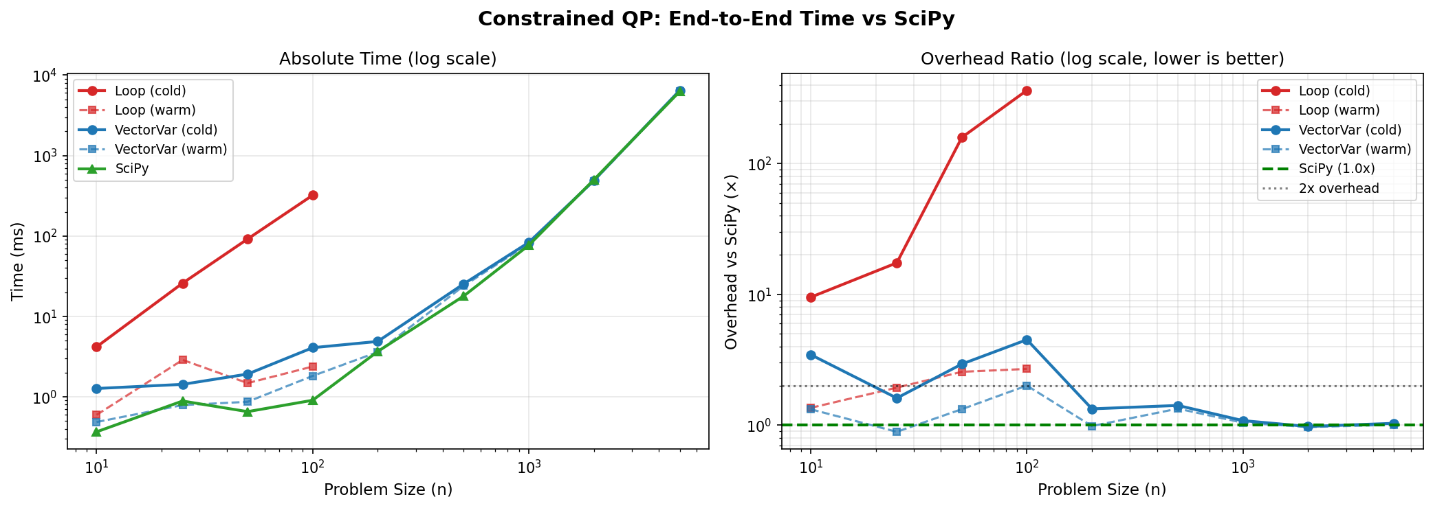
Objective: min Σx²ᵢ subject to Σxᵢ ≥ 1, xᵢ ≥ 0
1.5.1 VectorVariable with x.dot(x), x.sum()
| n | Build | Cold Solve | Warm Solve | SciPy | Cold Overhead | Warm Overhead |
|---|---|---|---|---|---|---|
| 10 | 0.1ms | 1.2ms | 0.6ms | 0.4ms | 3.6x | 1.7x |
| 25 | 0.0ms | 6.4ms | 0.9ms | 0.5ms | 13.7x | 2.0x |
| 50 | 0.0ms | 1.2ms | 0.7ms | 0.7ms | 1.8x | 1.1x |
| 100 | 0.0ms | 2.3ms | 1.5ms | 0.9ms | 2.5x | 1.6x |
| 200 | 0.0ms | 3.5ms | 2.5ms | 2.0ms | 1.8x | 1.3x |
| 500 | 0.0ms | 19.2ms | 14.9ms | 27.3ms | 0.7x | 0.5x |
| 1000 | 0.1ms | 96.0ms | 72.2ms | 78.3ms | 1.2x | 0.9x |
| 2000 | 0.1ms | 631.5ms | 560.6ms | 520.2ms | 1.2x | 1.1x |
| 5000 | 0.1ms | 7,392.2ms | 6,546.7ms | 6,382.6ms | 1.2x | 1.0x |
With O(1) Jacobian computation, constrained problems achieve near-parity with SciPy at scale (≤1.2x warm overhead for n ≥ 500).
1.6 MILP Scaling: Binary Knapsack
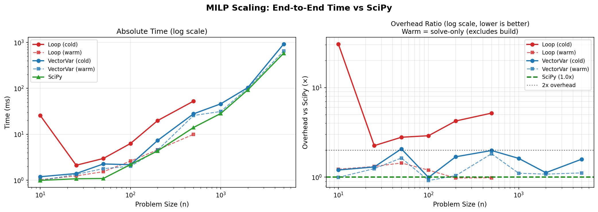
Problem: Single-constraint binary knapsack (sum(x) <= n//2)
1.6.1 VectorVariable (n ≤ 5,000)
| n | Build | Cold Solve | Warm Solve | SciPy | Cold Overhead | Warm Overhead |
|---|---|---|---|---|---|---|
| 10 | 0.0ms | 1.1ms | 1.0ms | 1.0ms | 1.2x | 1.0x |
| 25 | 0.1ms | 1.3ms | 1.3ms | 1.1ms | 1.3x | 1.2x |
| 50 | 0.0ms | 2.2ms | 1.8ms | 1.1ms | 2.1x | 1.6x |
| 100 | 0.0ms | 2.1ms | 2.0ms | 2.2ms | 1.0x | 0.9x |
| 200 | 0.0ms | 7.3ms | 4.5ms | 4.4ms | 1.7x | 1.0x |
| 500 | 0.0ms | 27.8ms | 25.7ms | 14.0ms | 2.0x | 1.8x |
| 1000 | 0.1ms | 45.8ms | 31.3ms | 28.3ms | 1.6x | 1.1x |
| 2000 | 0.1ms | 103.7ms | 100.0ms | 92.5ms | 1.1x | 1.1x |
| 5000 | 0.1ms | 922.1ms | 648.0ms | 580.4ms | 1.6x | 1.1x |
MILP warm solves achieve near-parity with SciPy at all scales. The integer programming solver adds minimal overhead beyond the SciPy milp baseline.
1.7 Overhead Summary by Problem Type
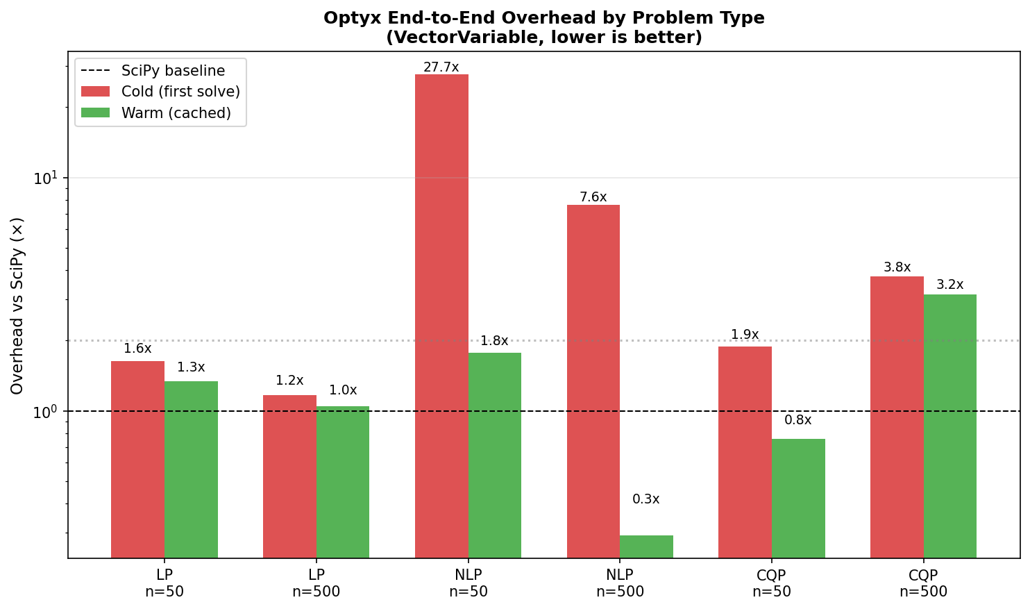
| Problem Type | Cold Overhead | Warm Overhead |
|---|---|---|
| LP (n=50) | 2.9x | 1.3x |
| LP (n=5000) | 2.3x | 1.1x |
| NLP (n=50) | 1.8x | 1.3x |
| NLP (n=5000) | 1.6x | 1.1x |
| CQP (n=50) | 1.8x | 1.1x |
| CQP (n=5000) | 1.2x | 1.0x |
| MILP (n=50) | 2.1x | 1.6x |
| MILP (n=5000) | 1.6x | 1.1x |
Pattern: LP, CQP, and MILP achieve near-parity with SciPy on warm solves at all scales. NLP overhead reflects autodiff costs on a trivially simple quadratic — for complex nonlinear problems, automatic differentiation eliminates the need for manual gradient derivation.
1.8 When to Use Optyx
1.8.1 Ideal Use Cases
✅ Parameter sweeps: Solve similar problems with different parameters
✅ Real-time optimization: Repeated solves with cached structure
✅ Prototyping: Clean Python API, no manual gradients
✅ Large LP: VectorVariable achieves parity with SciPy up to n=5,000
✅ Non-convex NLP: Automatic differentiation with exact gradients
✅ Mixed-integer programming: MILP at near-parity with SciPy milp
1.8.2 Consider Alternatives For
⚠️ One-shot problems: Cold-solve includes compilation overhead
⚠️ Large dense matrix problems (n>1000): CVXPY’s specialized solvers may scale better
⚠️ Loop-based variables at scale: Use VectorVariable instead
1.9 Running Benchmarks
# All benchmarks
uv run pytest benchmarks/ -v

# By category
uv run pytest benchmarks/validation/ -v
uv run pytest benchmarks/performance/ -v
uv run pytest benchmarks/accuracy/ -v
uv run pytest benchmarks/comparison/ -v

# Generate plots
uv run python benchmarks/run_benchmarks.py
1.10 Latest Console Summary
OVERHEAD SUMMARY BY PROBLEM TYPE
================================================================================
LP n=50: Cold=2.9x, Warm=1.3x
LP n=5000: Cold=2.3x, Warm=1.1x
NLP n=50: Cold=1.8x, Warm=1.3x
NLP n=5000: Cold=1.6x, Warm=1.1x
CQP n=50: Cold=1.8x, Warm=1.1x
CQP n=5000: Cold=1.2x, Warm=1.0x
MILP n=50: Cold=2.1x, Warm=1.6x
MILP n=5000: Cold=1.6x, Warm=1.1x

Saved: /workspaces/optix/benchmarks/results/overhead_breakdown.png

================================================================================